The Logistic Growth Equation Describes a Population That

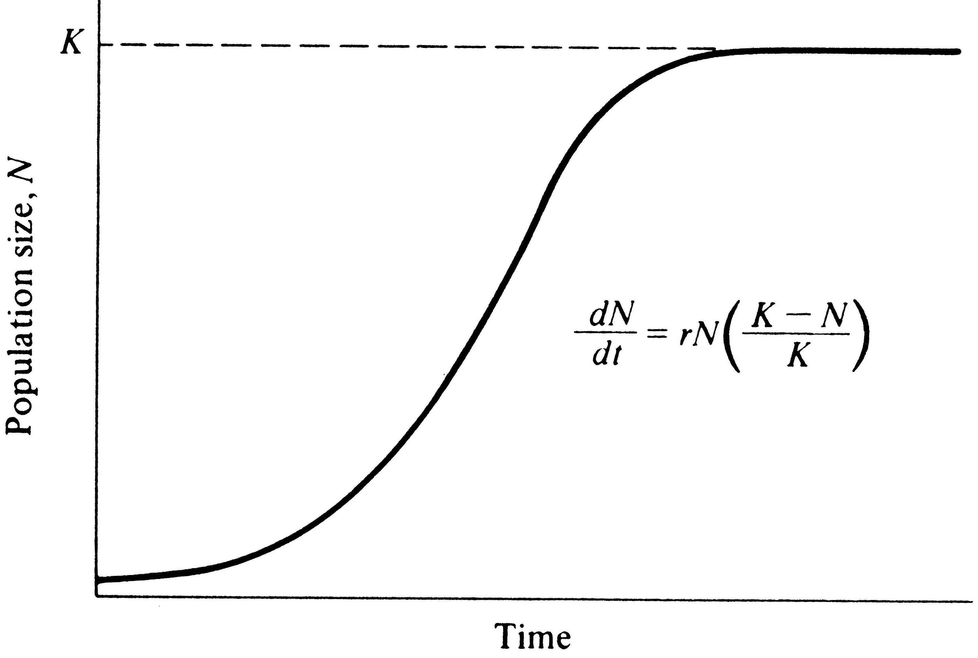
Per capita population growth and exponential growth. D N d t r N K N K where N population density at time t.

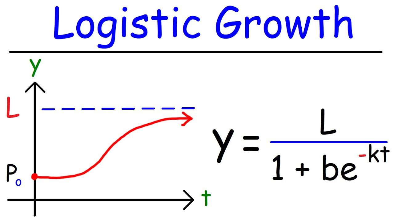
Logistic Growth Function And Differential Equations Youtube

The differential equation that describes logistic population growth is opkP1- where P is the population k 0 and M is the maximum sustainable population or carrying capacity.

. The Verhulst equation was published after Verhulst had read Thomas Malthus An Essay on the Principle of Population which describes the Malthusian growth model of simple unconstrained exponential growth. This is the logistic growth equation. Predation selects for later reproduction in guppies.

Assumptions of the logistic equation. Verhulst derived his logistic equation to describe the self-limiting growth of a biological population. Pt 10001 9e-016 - D.

Modeling Limited Population Growth with the Logistic Function Because of limits on food living space disease current technology war and other factors most populations have limited growth as opposed to unlimited exponential growth which is modeled by the classic exponential growth equation P P0btk. With P 1 5 0 0 P1500 P 1 5 0 0 and M 1 6 0 0 0 M16000 M 1 6 0 0 0 we get. Pt 10 1-09e-011 Verify.

K carrying capacity. Exponential logistic growth. Well start by plugging what we know into the logistic growth equation.

According to the logistic growth equation dNdtrmaxN K-NK A. This means that if the population starts at zero it will never change and if it starts at the carrying capacity it will never change. Population growth is zero when NK D.

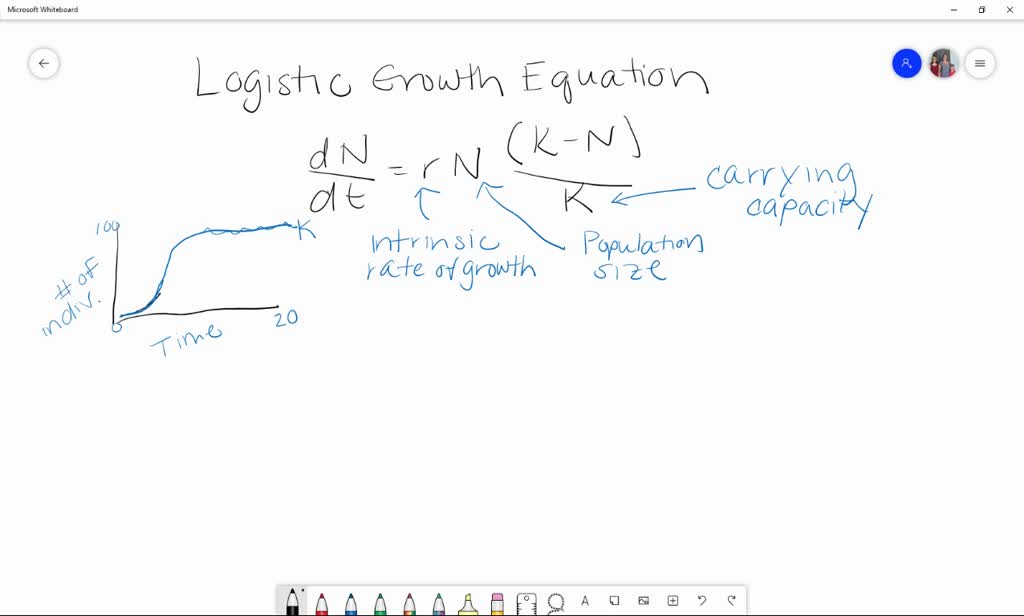
The most critical determinant of the life history strategy of guppies was the type of food they received. The corre-sponding equation is the so called logistic differential equation. Population ecologists usually use the symbol K for the carrying capacity so the intrinsic rate would be multiplied by K - N K.

Logistic Population Growth Model The initial value problem for logistic population growth 1 P0P0 K P kP dt dP has solution 0 where0 1 P K P A Ae K P t kt Here t the time the population grows P or Pt the population. A population that is declining in size and with further time may become extinct. A population that grows steadily when the.

Population growth rate based on birth and death rates. 3 birth and death rates change linearly with population size it is assumed that birth rates and. The formula we use to calculate logistic growth adds the carrying capacity as a moderating force in the growth rate.

R intrinsic rate of natural increase. 1 The carrying capacity is a constant. What does the logistic growth equation describe.

It is given by the following equation. Ronments impose limitations to population growth. A more accurate model postulates that the relative growth rate P0P decreases when P approaches the carrying capacity K of the environment.

Verhulst - Pearl Logistic growth is represented by the equation d t d N r N K K N what are a r b K. Pt 100e011 B. Substituting this Figure for the f N which is the function.

2 population growth is not affected by the age distribution. With regard to population growth rate when responses are limiting the plot is logistic. Logistic growth versus exponential growth.

The population grows exponentially when K is small. Rences A population that crashes after very rapid nearly exponential growth. The most critical determinant of the life history strategy of guppies was the concentration of calcium in the water.

We have reason to believe that it will be more realistic since the per capita growth rate is a decreasing function of the population. Rapidly overshoots the number the environment can support and then fluctuates around this number. Pt 100e -01t te-017 C.

DP dt kP µ 1 P K. The base growth rate isk and the logistic growth rate is kl 1 Notice that the logistic growth rate depends on P and so is variable over time. What is the solution to this logistic growth model.

Terms in this set 11 The logistic growth equation describes a population that. This is the currently selected item. The equation fracdPdt P0025 - 0002P is an example of the logistic equation and is the second model for population growth that we will consider.

Exponential and logistic growth in populations. Dp dt 01p 1 - 1000 p with the initial population p0 100. - The logistic growth equation describes logistic population growth - A change in growth rate that occurs as a function of population size - Logistic growth is density dependent - As a population approaches a habitats carrying capacity its growth rate should slow - r- and K-selected look different What are the 3 stages of density related growth.

The expression K N is indicative of how many individuals may be added to a population at a given stage and K N divided by K is the fraction of the carrying capacity available for further growth. Then the logistic differential equation is dP dt rP1 P K See this website for more information on the logistic equation. Now we need to find population after 5 5 5 years.

Represents the population of this organism as a function of time t and the constant P0 represents the initial population population of the organism at time t 0. The logistic equation is an autonomous differential equation so we can use the method of separation of variables. The per capita growth rate r increases as N approaches K C.

1 point A differential equation that describes logistic growth for some animal population is given by the formula. Multiple Choice ook A population that is increasing in size but never reaches its carrying capacity. Grows rapidly at small population sizes but whose growth rate slows and eventually stops as it reaches the number the environment can support.

Setting the right-hand side equal to zero gives P 0 and P 1072764. Population growth curve a when responses have not limited the growth the plot is exponential b when responses are limiting the growth the plot is logistic K is carrying capacity. The logistic equation can be solved by separation of.

The duck population after 2 2 2 years is 2 0 0 0 2000 2 0 0 0. The number of individuals added per unit time is greatest when N is close to zero B. An examination of the assumptions of the logistic equation explains why many populations display non-logistic growth patterns.

The Verhulst Pearl Logistic Growth Is Described To The Equation Dn Dt Rn K N K In This K Stand

9 Population Growth And Regulation

Solved According To The Logistic Growth Equation Frac D N D T R N Frac K N K A The Number Of Individuals Added Per Unit Time Is Greatest When N Is Close To Zero B The Per Capita